Plot a MAIHDA Group Comparison

Visualises the output of compare_maihda_groups as a point/forest plot of the VPC/ICC by group, as stacked variance-composition bars (between- vs within-stratum share) by group, as bars of the absolute between-stratum (intersectional) variance by group, or as bars of the additive share (PCV) by group. Dispatched via plot() on the classed result.

Usage

# S3 method for class 'maihda_group_comparison'
plot(
  x,
  type = c("vpc", "components", "between_variance", "pcv", "additive_share"),
  ...
)

Arguments

x

A maihda_group_comparison object from compare_maihda_groups.

type

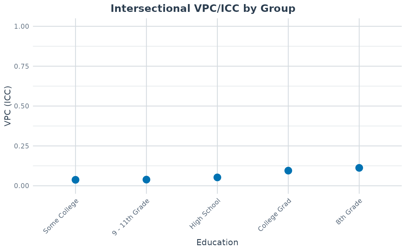
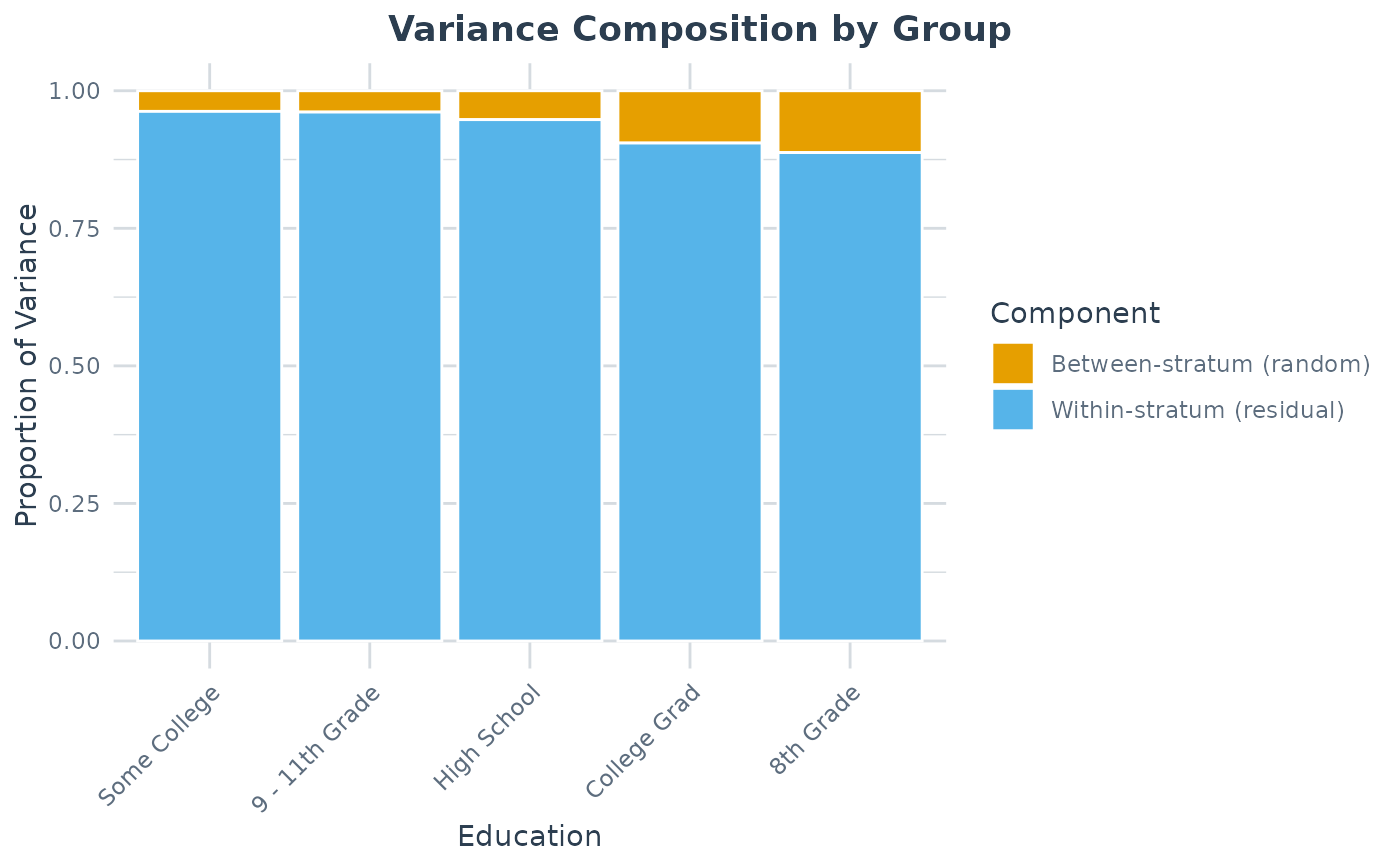
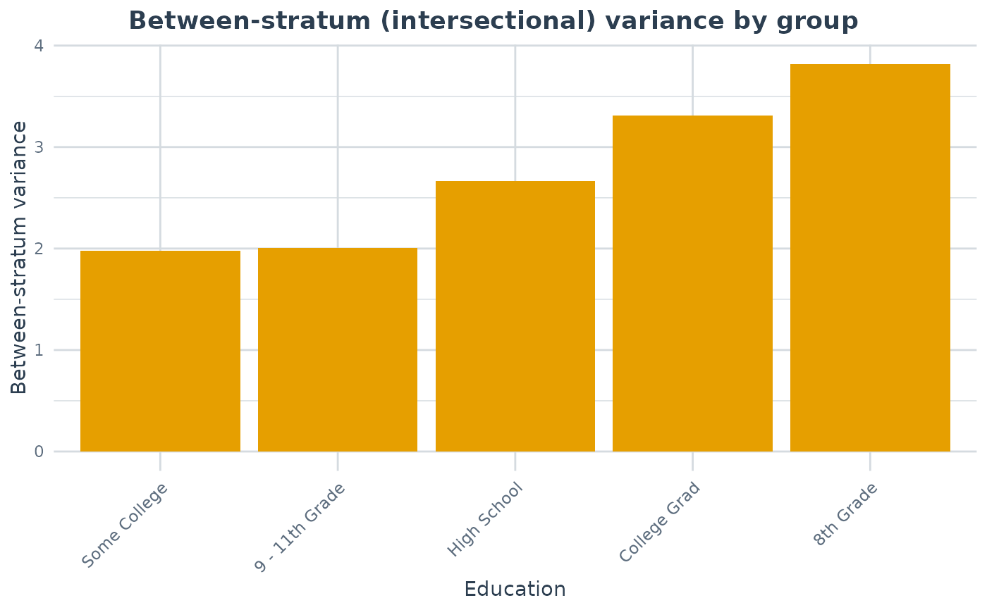
One of "vpc" (default) for VPC by group with optional bootstrap confidence intervals, "components" for stacked variance proportions (additive / interaction / residual for a crossed-dimensions comparison, between / other / residual otherwise), "between_variance" for the absolute between-stratum variance by group, "pcv" for the two-model additive share (null -> adjusted proportional change in between-stratum variance) by group, or "additive_share" for the crossed-dimensions additive share by group. The VPC is a share of the unexplained variance; "between_variance" shows the magnitude the ratio cannot convey (two groups with very different VPCs can share a between-stratum variance, and vice versa); "pcv" requires strata defined by at least two dimensions.

...

Additional arguments (not used).

Value

A ggplot2 object.

Examples

# \donttest{
data(maihda_health_data)
cmp <- compare_maihda_groups(BMI ~ Age + (1 | Gender:Race),
                             data = maihda_health_data, group = "Education")
#> boundary (singular) fit: see help('isSingular')
#> boundary (singular) fit: see help('isSingular')
plot(cmp, type = "vpc")

plot(cmp, type = "components")

plot(cmp, type = "between_variance")

# }