Longitudinal MAIHDA: intersectional inequalities over time

From a snapshot to a trajectory

Standard (cross-sectional) MAIHDA answers “do intersectional strata differ?” at a single point in time, summarised by the between-stratum VPC. With repeated measurements we can ask a richer question: “do strata differ in how they change over time?” – and decompose those trajectory differences into an additive part (the dimensions’ main effects and their interactions with time) and a multiplicative part (an intersectional trajectory beyond additive).

This is the longitudinal MAIHDA of Bell, Evans, Holman & Leckie (2024). It is a 3-level growth-curve model with measurement occasions (level 1) within individuals (level 2) within intersectional strata (level 3), with a random intercept and a slope on time at both the individual and stratum levels:

$y_{tij} = \beta_0 + \beta_1 t + \underbrace{(u_{0j} + u_{1j}\,t)}_{\text{stratum}} + \underbrace{(v_{0ij} + v_{1ij}\,t)}_{\text{individual}} + e_{tij}.$

Because the stratum random effect now has a slope, the between-stratum variance becomes a function of time:

$\operatorname{Var}_S(t) = \sigma^2_{u0} + 2t\,\sigma_{u01} + t^2 \sigma^2_{u1}, \qquad \operatorname{VPC}_S(t) = \frac{\operatorname{Var}_S(t)} {\operatorname{Var}_S(t) + \operatorname{Var}_I(t) + \sigma^2_e}.$

The data

The bundled maihda_long_data is a simulated panel: 600 people, each measured over five waves, within 12 strata of gender $\times$ ethnicity $\times$ education. The trajectory differences are constructed to be mostly additive with one genuine interaction, so the decomposition below is interpretable.

data(maihda_long_data)
head(maihda_long_data)
#>      id wave gender ethnicity education age wellbeing low_wellbeing
#> 1 P0001    0    Men      EthB       Low  50     3.732             1
#> 2 P0001    1    Men      EthB       Low  50     3.696             1
#> 3 P0001    2    Men      EthB       Low  50     1.638             1
#> 4 P0001    3    Men      EthB       Low  50     3.585             1
#> 5 P0001    4    Men      EthB       Low  50     3.594             1
#> 6 P0002    0  Women      EthB       Low  56     5.631             0

It is long format, one row per person-occasion, with a person id (id) and a numeric time (wave).

Fitting and the time-varying VPC

Supply id and time to fit_maihda(). You only need to write the strata shorthand (1 | var1:var2); the growth slopes on time are added for you.

m <- fit_maihda(wellbeing ~ wave + (1 | gender:ethnicity:education),
                data = maihda_long_data, id = "id", time = "wave")
#> Warning in checkConv(attr(opt, "derivs"), opt$par, ctrl = control$checkConv, : Model failed to converge with max|grad| = 0.00213664 (tol = 0.002, component 1)
#>   See ?lme4::convergence and ?lme4::troubleshooting.
summary(m)
#> MAIHDA Model Summary
#> ====================
#> 
#> Fit diagnostics:
#>   Convergence warnings reported by lme4:
#>     - Model failed to converge with max|grad| = 0.00213664 (tol = 0.002, component 1)
#>   See ?lme4::convergence and ?lme4::troubleshooting.
#> 
#> 
#> Variance Partition Coefficient (VPC/ICC) at baseline (wave = 0):
#>   Estimate: 0.3986
#> 
#> Variance Components:
#>                                            component  variance     sd
#>                Between-stratum: intercept (time = 0)  0.407878 0.6387
#>                        Between-stratum: slope (wave)  0.042860 0.2070
#>          Between-stratum: intercept-slope covariance  0.088498     NA
#>        Between-individual (id): intercept (time = 0)  0.255609 0.5056
#>                Between-individual (id): slope (wave)  0.019360 0.1391
#>  Between-individual (id): intercept-slope covariance -0.001107     NA
#>                                    Within (residual)  0.359816 0.5998
#> 
#> Time-varying VPC/ICC (between-stratum share over wave):
#>   range 0.3986 to 0.6629 across wave in [0, 4].
#>   The between-stratum variance is a function of time (random intercept +
#>   slope), so the VPC varies; it depends on where time is zeroed. See
#>   plot(type = "vpc_trajectory") for the full curve.
#> 
#> Fixed Effects:
#>         term  estimate
#>  (Intercept)  4.986466
#>         wave -0.006306
#> 
#> Stratum baseline (intercept) deviations (first 10):
#>  stratum stratum_id               label random_effect      se lower_95 upper_95
#>        1          1    Men × EthB × Low      -0.63796 0.08953 -0.81344  -0.4625
#>        2          2  Women × EthB × Low      -0.06459 0.08595 -0.23305   0.1039
#>        3          3   Men × EthA × High       0.86072 0.07783  0.70819   1.0133
#>        4          4   Men × EthB × High       0.09121 0.10260 -0.10988   0.2923
#>        5          5 Women × EthA × High       0.93602 0.08804  0.76345   1.1086
#>        6          6 Women × EthC × High       0.35851 0.13545  0.09302   0.6240
#>        7          7   Men × EthC × High      -0.11460 0.13287 -0.37503   0.1458
#>        8          8    Men × EthA × Low      -0.32848 0.07050 -0.46667  -0.1903
#>        9          9  Women × EthA × Low       0.15992 0.07326  0.01633   0.3035
#>       10         10    Men × EthC × Low      -0.82710 0.13287 -1.08753  -0.5667
#>   ... and 2 more strata
#>   (random slope not shown; use predict(type = "strata") for the per-stratum intercept and slope, or plot(type = "trajectories")).

summary() reports the VPC at the baseline (reference time, the earliest wave) and the full trajectory of the VPC across the observed times. Plot it:

plot(m, type = "vpc_trajectory")   # VPC(t), with the reference time marked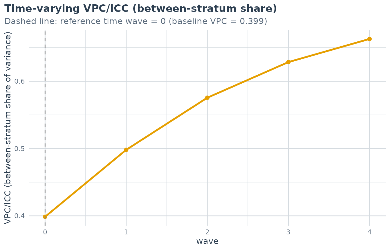

plot(m, type = "trajectories")     # predicted per-stratum mean trajectories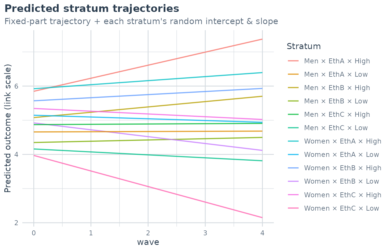

A rising VPC trajectory means the strata fan out over time (intersectional inequality grows).

Decomposing the trajectory: additive vs. multiplicative

maihda(decomposition = "longitudinal") (selected automatically when id/time are supplied) fits a null growth model and an adjusted growth model. The adjusted model adds the dimensions’ main effects and their interactions with time (dim:time), so the stratum-level variance it leaves behind is the interaction beyond additive.

a <- maihda(wellbeing ~ wave + (1 | gender:ethnicity:education),
            data = maihda_long_data, id = "id", time = "wave",
            decomposition = "longitudinal")
#> Warning in checkConv(attr(opt, "derivs"), opt$par, ctrl = control$checkConv, : Model failed to converge with max|grad| = 0.00213664 (tol = 0.002, component 1)
#>   See ?lme4::convergence and ?lme4::troubleshooting.
a$pcv
#> Longitudinal PCV (additive vs. multiplicative intersectionality)
#> ================================================================
#> 
#> Baseline (wave = 0) variance: 0.4079 (null) -> 0.0332 (adjusted)
#>   PCV_intercept: 91.9% of the baseline between-stratum inequality is additive.
#> Slope (wave) variance:          0.0429 (null) -> 0.0058 (adjusted)
#>   PCV_slope:     86.6% of the *trajectory* between-stratum inequality is additive
#>                  (the remainder is the multiplicative/interaction part).
#> 
#> The PCV is the share of the null model's between-stratum (trajectory) variance
#> explained by the dimensions' additive main effects and their time interactions;
#> a high PCV_slope means trajectory inequalities are 'mostly additive'.
#>

The PCV is reported separately for the two pieces of the trajectory:

PCV_intercept – the share of the baseline between-stratum inequality explained by the additive main effects.
PCV_slope – the share of the trajectory (slope) between-stratum inequality explained additively. A high PCV_slope is the “trajectories are mostly additive” finding; the remainder is the multiplicative/interaction part.

plot(a, type = "pcv_trajectory")   # the additive share over time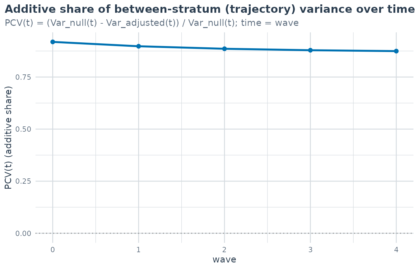

Scope and cautions

Identifiability. A stratum random slope needs enough occasions per stratum; sparse strata or few waves can give a singular lme4 fit (surfaced in the fit diagnostics) – the brms engine handles this better.
Not a single number. The VPC is time-varying, so extract_between_variance() and calculate_pvc() deliberately refuse a longitudinal model; use the longitudinal decomposition above.
Out of scope (v1). Design-weighted, contextual (stratum $\times$ place $\times$ time), and wemix/ordinal longitudinal models are not yet supported.

Reference

Bell, A., Evans, C., Holman, D., & Leckie, G. (2024). Extending intersectional multilevel analysis of individual heterogeneity and discriminatory accuracy (MAIHDA) to study individual longitudinal trajectories, with application to mental health in the UK. Social Science & Medicine, 351, 116955. doi:10.1016/j.socscimed.2024.116955