Order-Invariant PCV Attribution Across Predictors (Shapley / Dominance)

Apportions the between-stratum variance reduction (the PCV) among a set of predictors. Where stepwise_pcv adds the variables one at a time – so each variable's contribution depends on its entry order – pcv_importance() treats the PCV as a value function over variable subsets and attributes it fairly: the flagship "shapley" method averages each variable's marginal PCV over every possible entry order, and "dominance" adds Budescu's pairwise dominance detail (its general dominance weights coincide with the Shapley values). All methods satisfy the efficiency identity: the contributions sum exactly to the full model's total PCV. (The order-dependent "sequential" method is deprecated; use stepwise_pcv for the sequential path – see the method argument.)

Two attribution targets are useful in a MAIHDA. Passing the stratum dimensions (e.g. c("gender", "race", "education")) splits the additive share – the canonical null-to-adjusted PCV – fairly across the dimensions: which social dimension drives the additive between-stratum inequality. Passing individual-level covariates gives an order-invariant counterpart to stepwise_pcv(): how much each covariate explains of the between-stratum variance (subject to the latent-scale caveat below for non-Gaussian families).

Usage

pcv_importance(
  data,
  outcome,
  vars,
  method = c("shapley", "sequential", "dominance"),
  approx = c("exact", "montecarlo"),
  n_perm = 2000,
  engine = "lme4",
  family = "gaussian",
  context = NULL,
  sampling_weights = NULL,
  bootstrap = FALSE,
  n_boot = 1000,
  conf_level = 0.95,
  estimation = c("fitted", "ML")
)

Arguments

data: Data frame with observations. Ensure make_strata was run first so the stratum variable exists.
outcome: Character string; the dependent variable.
vars: Character vector of predictors (stratum dimensions and/or covariates) among which the PCV is apportioned. Order does not affect the "shapley" and "dominance" results; it defines the path for "sequential".
method: Attribution method: "shapley" (default; order-invariant Shapley values) or "dominance" (Budescu dominance analysis: general dominance – equal to the Shapley values – plus the conditional and complete dominance detail). "sequential" (the order-dependent one-at-a-time path) is deprecated and will be removed in a future release: it still runs but warns, and stepwise_pcv is the supported sequential decomposition – it additionally reports the step-specific Step_PCV and, for a binary outcome, the discriminatory-accuracy trajectory (AUC, MOR).
approx: For method = "shapley" only: "exact" fits all \(2^k - 1\) non-empty variable subsets (plus the null); "montecarlo" samples n_perm random entry orders instead. When approx is not supplied it defaults to "exact" for up to 10 variables and switches to "montecarlo" (with a message) beyond. "sequential" needs only the \(k\) path models and ignores approx; "dominance" requires every subset, so it errors if approx = "montecarlo" is requested.
n_perm: Number of random permutations for approx = "montecarlo". Default 2000. Distinct subset fits are cached, so the number of model fits is bounded by min(2^k, n_perm * (k - 1) + k + 1); set a seed (set.seed()) for reproducible sampling.
engine: Modeling engine ("lme4", "brms", "wemix", or "ordinal"); default "lme4". Resolved exactly as in stepwise_pcv: switches to "wemix" when sampling_weights is supplied and to "ordinal" for an ordinal family or ordered-factor outcome. Exact attribution with engine = "brms" refits a Stan model for every subset and is strongly discouraged beyond a handful of variables (see Details).
family: Error distribution and link function. Default "gaussian"; a binary or ordered-factor outcome is auto-detected when family is left unspecified, mirroring stepwise_pcv.
context: Optional higher-level context column(s) (e.g. "school"), forwarded to every subset fit so each model carries the crossed (1 | context) intercept alongside the stratum effect; the attribution is then of the between-stratum PCV net of the context, exactly as in stepwise_pcv. lme4/brms engines only.
sampling_weights: Optional name of a sampling-weight column for design-weighted fits; see fit_maihda. The weight column joins the complete-case filter so every subset fit uses the same analytic sample.
bootstrap: Logical; compute parametric-bootstrap confidence intervals for each contribution by refitting every subset model on responses simulated from the full model. lme4 engine and exact attribution only; the cost is n_boot times the number of subset models (up to n_boot * 2^k refits). Default FALSE.
n_boot: Number of bootstrap draws if bootstrap = TRUE. Default 1000.
conf_level: Confidence level for bootstrap intervals. Default 0.95.
estimation: Variance-estimation basis for the between-stratum variances the attribution differences across subset models, "fitted" (default) or "ML"; see calculate_pcv. Affects Gaussian lmer fits only.

Value

An object of class maihda_pcv_importance: a list with

importance: Data frame with one row per variable (in the order of vars): Contribution (the variable's share of the total PCV, on the PCV scale), Share (Contribution / total_pcv; NA when the total PCV is zero), plus MC_SE (Monte-Carlo standard errors, approx = "montecarlo" only) and CI_lower/CI_upper (bootstrap = TRUE only).
total_pcv: The full-model PCV, \((V_0 - V_{full}) / V_0\); the contributions sum to this value (efficiency).
null_variance, full_variance: Between-stratum variance of the null and the full (all-vars) model.
subsets: Data frame of every subset model fit: the variables in the subset, its size, between-stratum variance, and PCV \(v(S)\).
conditional, complete_dominance: method = "dominance" only: the conditional dominance matrix (variables x adjustment-set size) and the pairwise complete-dominance matrix.
method, approx, n_perm, n_fits, n_obs, engine, family, context, bootstrap, conf_level, n_boot_ok, n_boot_boundary, n_boot_nonconverged, estimation, estimation_used: Metadata; n_fits counts the distinct models fit (including the null), n_boot_ok the number of successful bootstrap draws, n_boot_boundary the draws excluded because the null between-stratum variance hit the zero boundary (the intervals are then conditional on a positive null variance), n_boot_nonconverged the retained draws whose refit optimiser did not converge, estimation is the variance-estimation basis ("fitted"/"ML") requested for every subset model's between-stratum variance, and estimation_used is the basis actually used ("mixed" when an ML refit was skipped at the boundary, leaving a subset model on REML).

Details

Value function and efficiency. Write \(V_0\) for the null model's between-stratum variance and \(V(S)\) for the between-stratum variance after adding the variable subset \(S\) as fixed effects (each put on the estimation basis – the default "fitted" keeps each lmer fit's own REML variance, "ML" refits it with maximum likelihood – exactly as in calculate_pcv and stepwise_pcv, so all attributions live on the same scale as the rest of the package). The value function is \(v(S) = (V_0 - V(S)) / V_0\) – the total PCV of the model that adds \(S\) – and the Shapley contribution of variable \(i\) averages its marginal PCV \(v(S \cup \{i\}) - v(S)\) over all subsets with the usual Shapley weights. Because every permutation's marginals telescope to \(v(N)\), the contributions of every method here (including the Monte-Carlo approximation, for any n_perm) sum exactly to the full-model total PCV. This is the multilevel-PCV analogue of the LMG / Shorrocks-Shapley decomposition of \(R^2\) (Groemping 2006; Shorrocks 2013).

Sequential method (deprecated) vs. stepwise_pcv(). The "sequential" method is deprecated in favour of stepwise_pcv, which owns the sequential trajectory and also reports the Step_PCV column and the discriminatory-accuracy path. While it remains, its contributions are the increments in total PCV along the entry order, \(v(\{x_1..x_i\}) - v(\{x_1..x_{i-1}\})\) – i.e. diff(c(0, Total_PCV)) of the stepwise_pcv table, so they sum to the same total. They are not the Step_PCV column, which normalises each step by the previous step's variance rather than by \(V_0\).

Exact vs. Monte-Carlo cost. The exact attribution fits \(2^k - 1\) non-empty subset models plus the null – \(2^k\) fits in total, with every fit cached and reused across all marginal differences: 256 fits at \(k = 8\), 1024 at \(k = 10\). That is feasible for lme4 but quickly infeasible beyond, and each of those fits is a separate Stan run under engine = "brms" – exact attribution on brms is therefore strongly discouraged except for very small \(k\). The Monte-Carlo route samples n_perm entry orders (unbiased for the Shapley values, since a uniform random permutation reproduces the Shapley weights), reports a per-variable Monte-Carlo standard error, and warns when the largest MC_SE exceeds 0.01 on the PCV scale (increase n_perm).

Latent-scale families and rescaling. For binomial/ordinal (and, in attenuated form, count) families, adding a predictor that varies within strata rescales the latent metric, so its marginal PCV mixes explained variance with rescaling (see the latent-scale note in calculate_pcv); Shapley values of the PCV inherit this. Attribution among the stratum dimensions – constant within each stratum – is largely unaffected.

Suppression and negative contributions. The PCV can be negative, so a contribution (and its Share) can be negative or exceed 100%. Efficiency still holds; contributions are reported signed and no non-negative normalisation is applied. A negative Shapley contribution flags a suppressor-style variable whose inclusion tends to raise the between-stratum variance.

Bootstrap. With bootstrap = TRUE the whole attribution is bootstrapped: responses are simulated from the full model and every subset model is refit per draw (lme4::refit), giving percentile intervals per contribution – n_boot times n_fits refits, so gate it by cost. Available for engine = "lme4" with exact attribution (any method); the Monte-Carlo approximation already carries its own sampling error and is not combined with the bootstrap. As in calculate_pcv, refit() holds a glmer.nb dispersion parameter fixed at its original estimate.

Reproducibility

approx = "montecarlo" draws random permutations with the session RNG; call set.seed() first for reproducible results. The exact methods are deterministic.

References

Budescu, D. V. (1993). Dominance analysis: a new approach to the problem of relative importance of predictors in multiple regression. Psychological Bulletin, 114(3), 542-551.

Groemping, U. (2006). Relative importance for linear regression in R: the package relaimpo. Journal of Statistical Software, 17(1), 1-27.

Shorrocks, A. F. (2013). Decomposition procedures for distributional analysis: a unified framework based on the Shapley value. Journal of Economic Inequality, 11, 99-126.

Examples

# \donttest{
strata <- make_strata(maihda_sim_data, c("gender", "race"))

# Order-invariant split of the PCV across the two dimensions and age
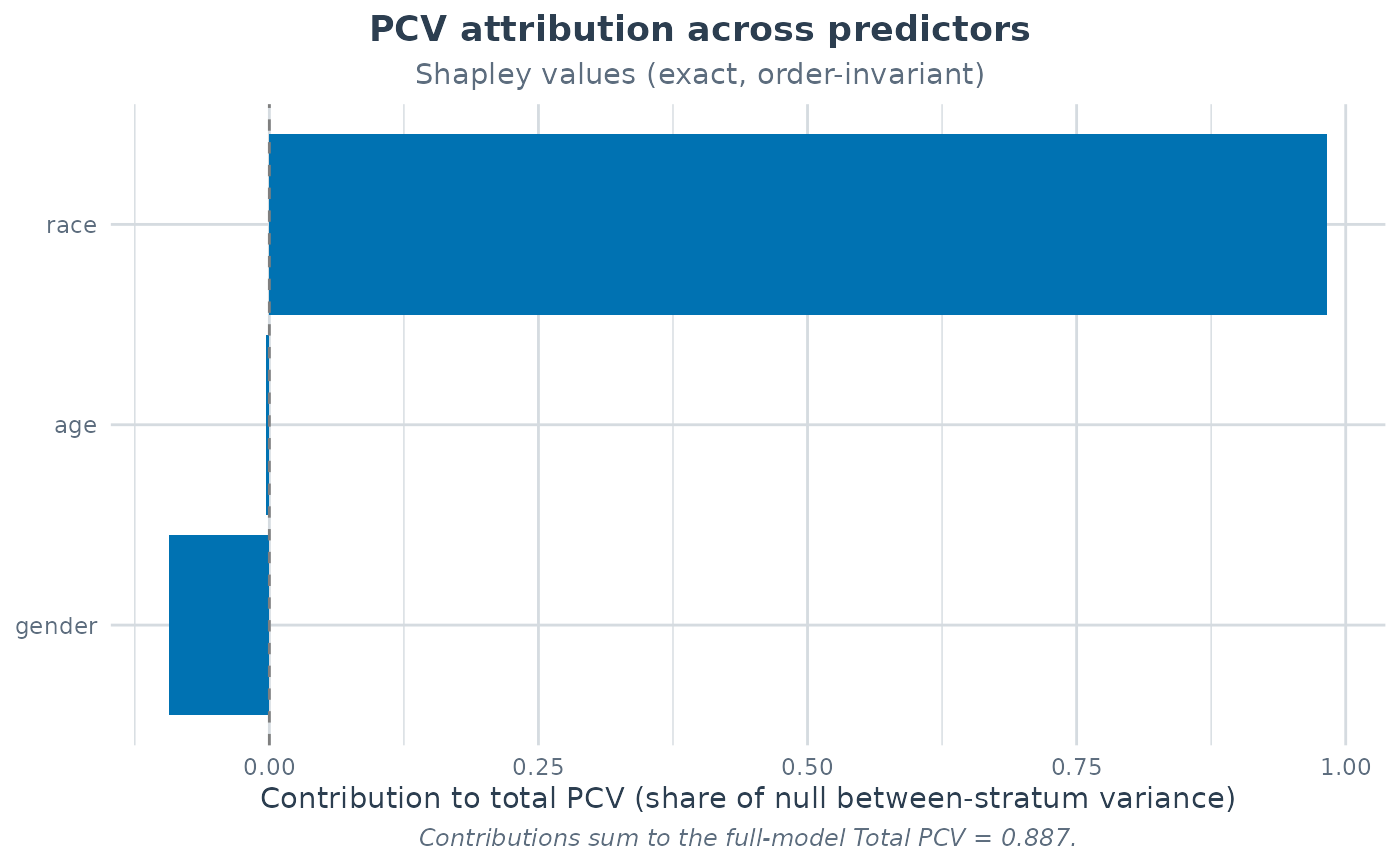
imp <- pcv_importance(strata$data, "health_outcome", c("gender", "race", "age"))
print(imp)
#> PCV Attribution Across Predictors
#> =================================
#> 
#> Method:  Shapley values (exact)
#> Outcome: health_outcome   Engine: lme4 (gaussian(identity))
#> Analytic sample: 500 observations; 8 models fit (incl. null).
#> Variance basis: as fitted (REML for Gaussian lmer, matching summary())
#> 
#> Between-stratum variance: null 26.714703 -> full model 3.031709
#> Total PCV (null -> all variables): 0.8865
#> 
#>  Variable Contribution   Share
#>    gender      -0.0934  -10.5%
#>      race       0.9830 +110.9%
#>       age      -0.0031   -0.3%
#>     Total       0.8865  100.0%
#> 
#> Contributions are shares of the null model's between-stratum variance
#> explained (the PCV scale) and sum to the full-model Total PCV (efficiency).
#> Negative contributions flag suppression: the variable tends to RAISE the
#> between-stratum variance; signed values are reported (no normalisation).
#> 
plot(imp)


# Dominance analysis: adds conditional / complete dominance detail
pcv_importance(strata$data, "health_outcome", c("gender", "race", "age"),
               method = "dominance")
#> PCV Attribution Across Predictors
#> =================================
#> 
#> Method:  Dominance analysis (general dominance = Shapley)
#> Outcome: health_outcome   Engine: lme4 (gaussian(identity))
#> Analytic sample: 500 observations; 8 models fit (incl. null).
#> Variance basis: as fitted (REML for Gaussian lmer, matching summary())
#> 
#> Between-stratum variance: null 26.714703 -> full model 3.031709
#> Total PCV (null -> all variables): 0.8865
#> 
#>  Variable Contribution   Share
#>    gender      -0.0934  -10.5%
#>      race       0.9830 +110.9%
#>       age      -0.0031   -0.3%
#>     Total       0.8865  100.0%
#> 
#> Contributions are shares of the null model's between-stratum variance
#> explained (the PCV scale) and sum to the full-model Total PCV (efficiency).
#> Negative contributions flag suppression: the variable tends to RAISE the
#> between-stratum variance; signed values are reported (no normalisation).
#> 
#> Conditional dominance (average marginal PCV by adjustment-set size):
#>         size_0  size_1  size_2
#> gender -0.1553 -0.0907 -0.0344
#> race    0.9336  0.9858  1.0297
#> age     0.0167 -0.0003 -0.0257
#> Complete dominance: race > gender, race > age, age > gender

# Monte-Carlo approximation (set a seed for reproducibility)
set.seed(42)
pcv_importance(strata$data, "health_outcome", c("gender", "race", "age"),
               approx = "montecarlo", n_perm = 500)
#> PCV Attribution Across Predictors
#> =================================
#> 
#> Method:  Shapley values (Monte-Carlo, 500 permutations)
#> Outcome: health_outcome   Engine: lme4 (gaussian(identity))
#> Analytic sample: 500 observations; 8 models fit (incl. null).
#> Variance basis: as fitted (REML for Gaussian lmer, matching summary())
#> 
#> Between-stratum variance: null 26.714703 -> full model 3.031709
#> Total PCV (null -> all variables): 0.8865
#> 
#>  Variable Contribution   Share  MC_SE
#>    gender      -0.0888  -10.0% 0.0029
#>      race       0.9798 +110.5% 0.0027
#>       age      -0.0046   -0.5% 0.0009
#>     Total       0.8865  100.0%       
#> 
#> Contributions are shares of the null model's between-stratum variance
#> explained (the PCV scale) and sum to the full-model Total PCV (efficiency).
#> Negative contributions flag suppression: the variable tends to RAISE the
#> between-stratum variance; signed values are reported (no normalisation).
#> 
# }