
Creates various plots for visualizing MAIHDA model results including variance partition coefficient comparisons, observed vs. shrunken estimates, and predicted subgroup values with conditional intervals.
Usage
# S3 method for class 'maihda_model'
plot(
  x,
  type = c("all", "vpc", "obs_vs_shrunken", "predicted", "upset", "effect_decomp",
    "prediction_deviation", "context_vpc", "vpc_trajectory", "trajectories"),
  summary_obj = NULL,
  n_strata = 50,
  highlight_interactions = FALSE,
  only_flagged = FALSE,
  highlight_by = c("flag", "rope"),
  rope = NULL,
  select = c("order", "deviation"),
  order_by = c("predicted_desc", "stratum", "predicted_asc", "deviation", "size"),
  quantity = c("predicted", "interaction"),
  ...
)
Arguments
- x
A maihda_model object from
fit_maihda().- type
Character string specifying plot type:
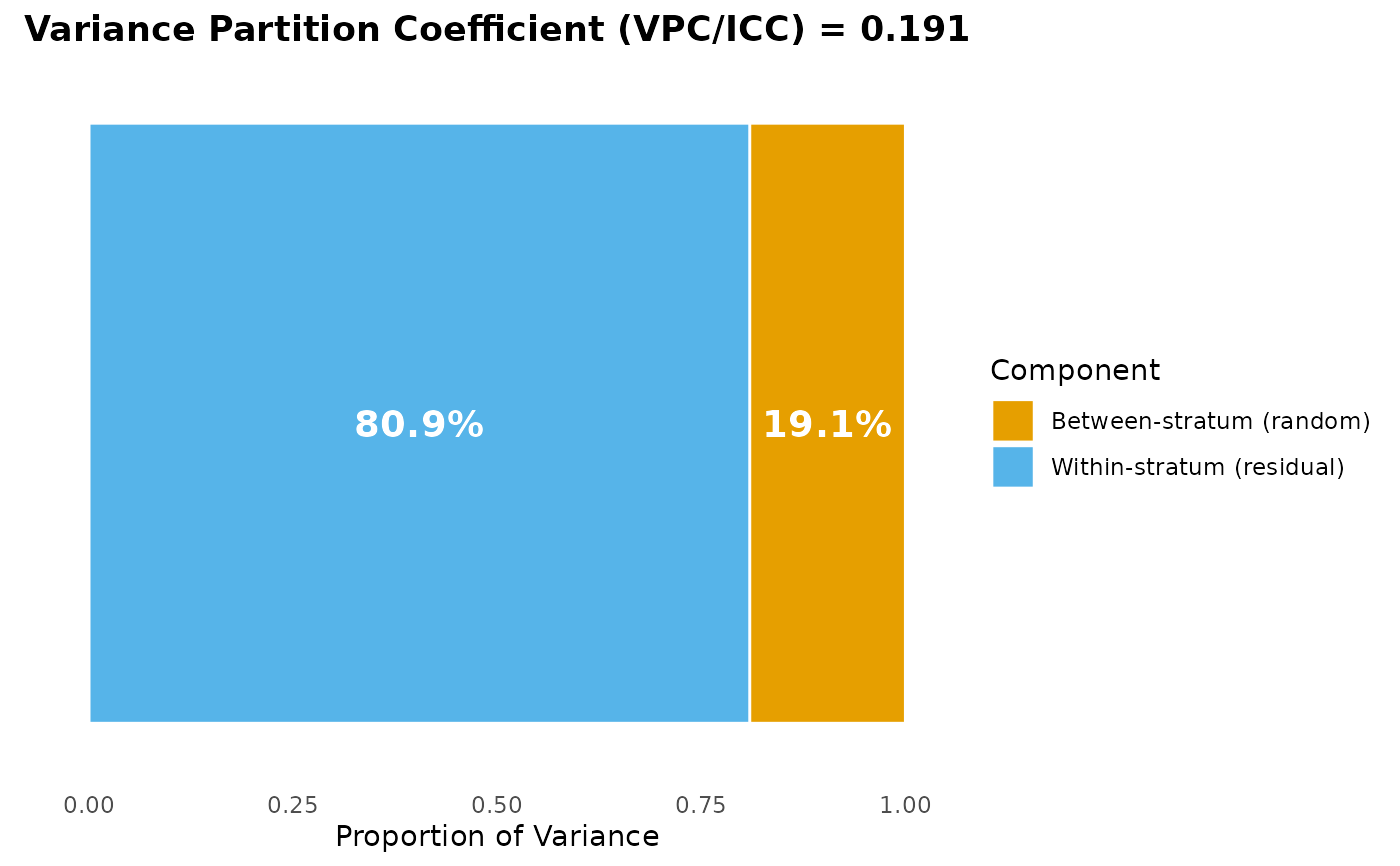
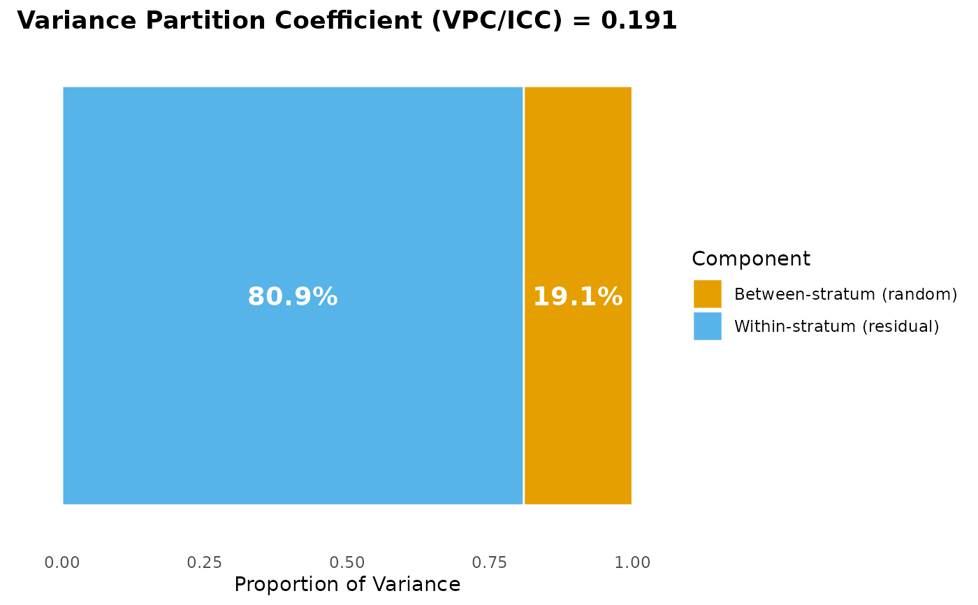
"vpc": Variance partition coefficient visualization
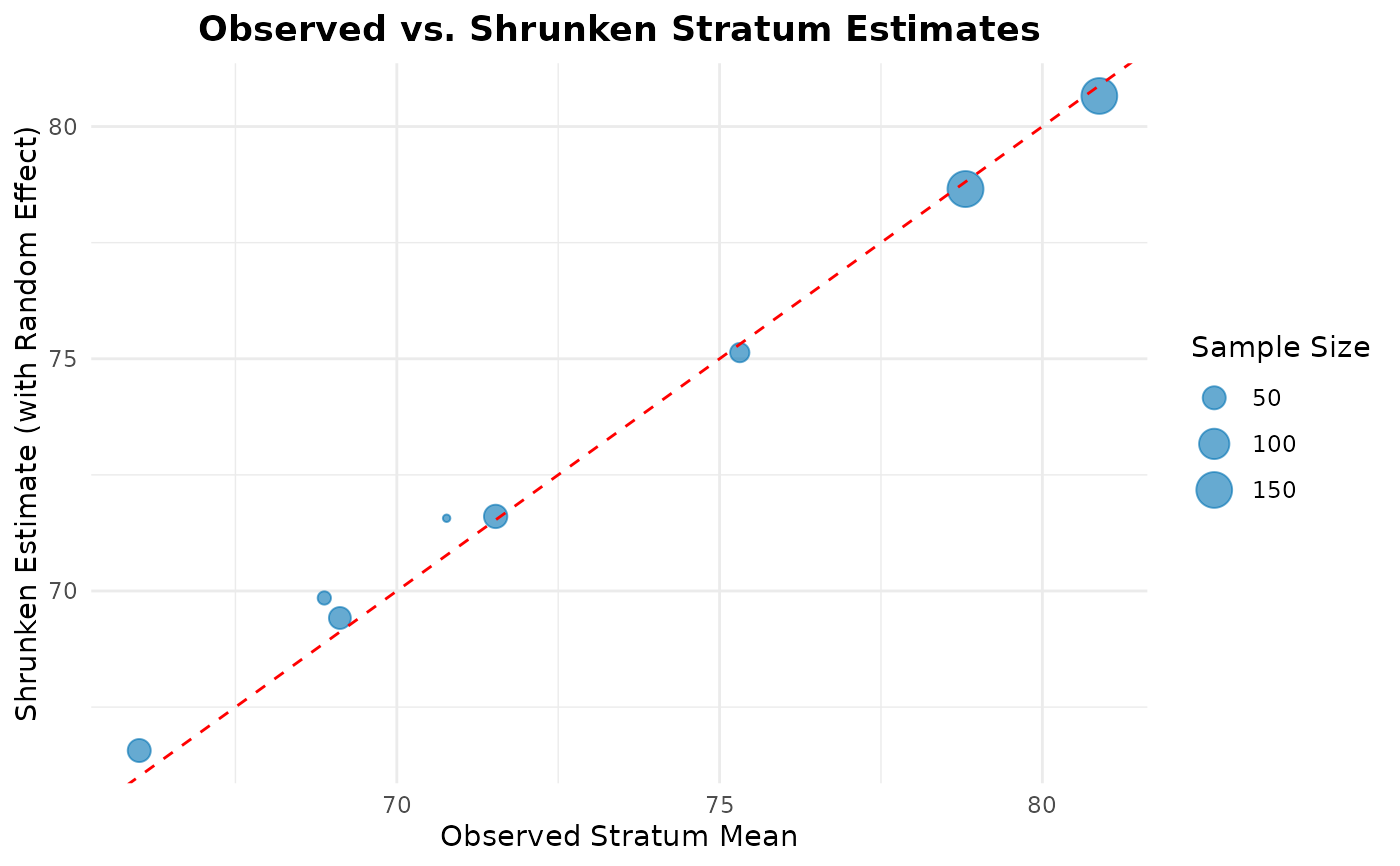
"obs_vs_shrunken": Observed vs. shrunken stratum means. The y-axis (model-based estimate) includes the fixed effects, so for a covariate-adjusted model the distance from the diagonal reflects both shrinkage and covariate adjustment, not shrinkage alone; it is a pure shrinkage view only for an intercept-only (null) model
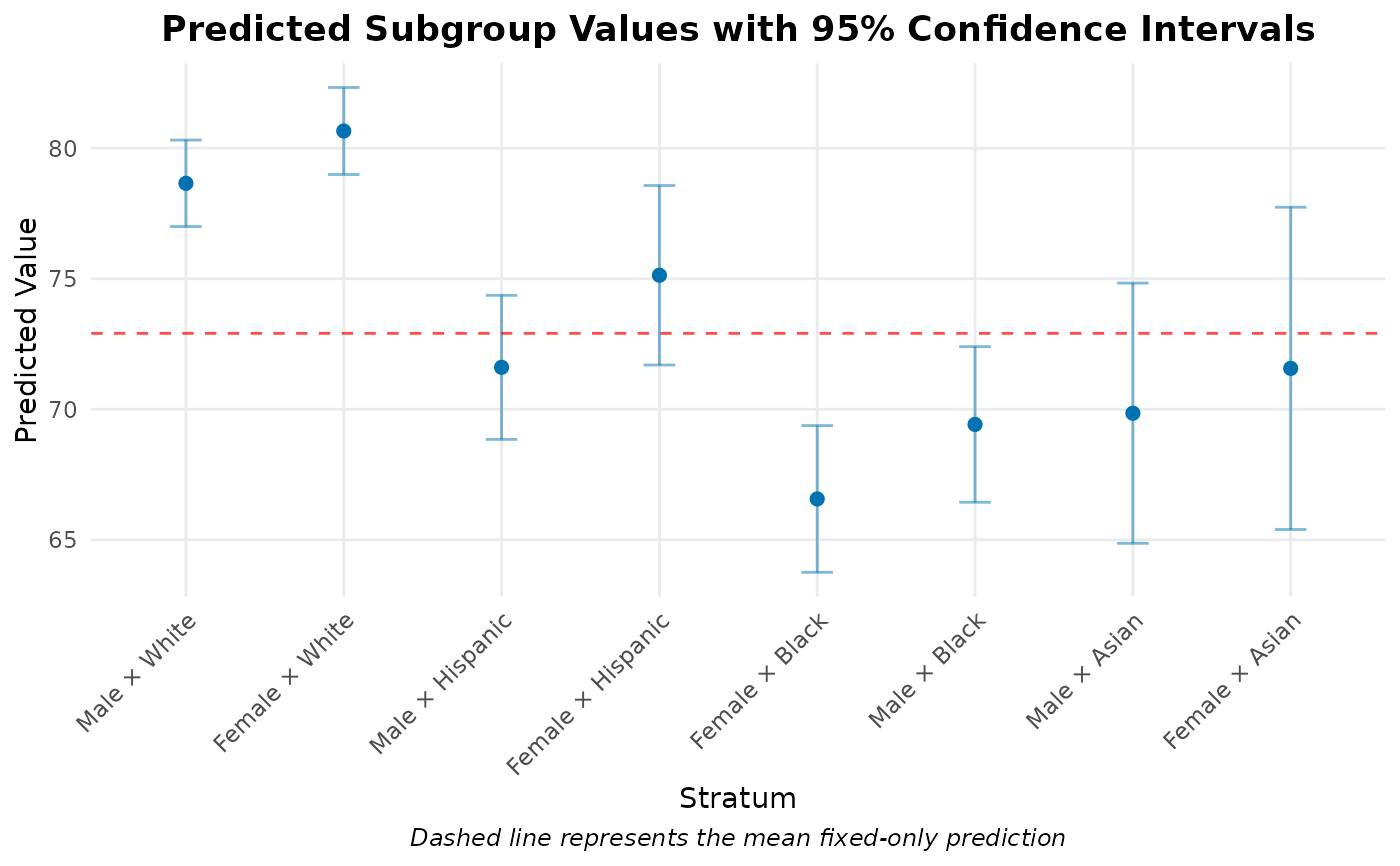
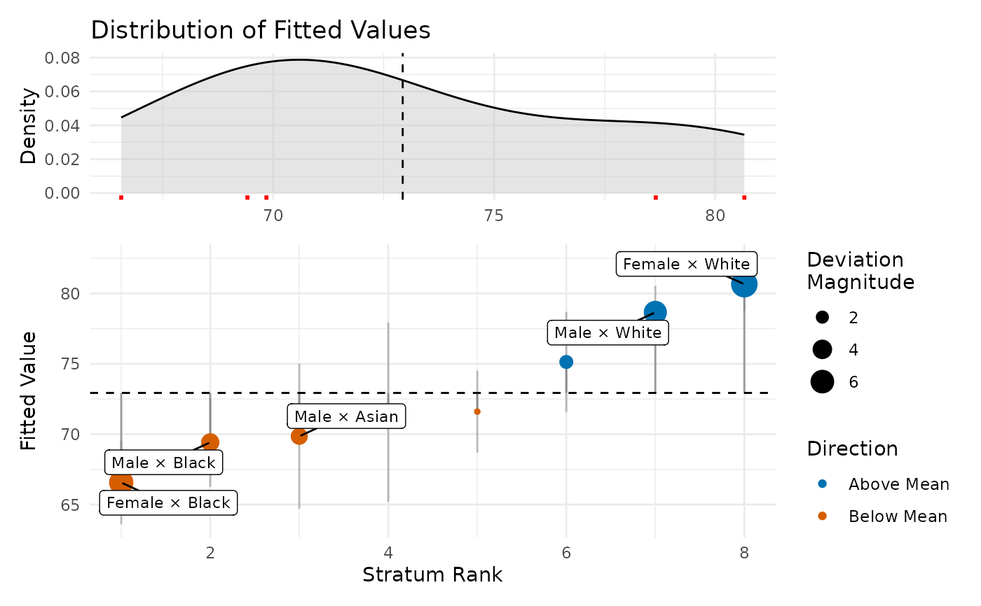
"predicted": Predicted values for each stratum with conditional (random-effect) intervals: the stratum random effect's own interval – a Wald interval on the conditional SD of the BLUP for the likelihood engines, the posterior interval of \(u_j\) for brms – shifted onto the outcome scale by the fixed-effect prediction, which is held at its point estimate. They answer “does this stratum depart from the dashed across-strata reference?”, which is what a caterpillar plot is read for; they are not intervals for the predicted value itself. Holding the fixed effects at a point estimate stops the fixed-effect uncertainty carried inside the random-effect interval from cancelling against the random effect it is correlated with, so these intervals are wider than a full interval for the stratum's predicted outcome, markedly so when there are few strata. By default the strata are ordered highest-to-lowest predicted value (a ranked caterpillar plot); see
order_byto change or disable the ordering"upset": UpSet-style alternative to
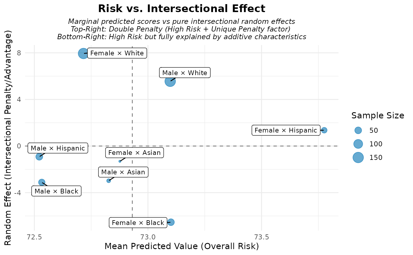
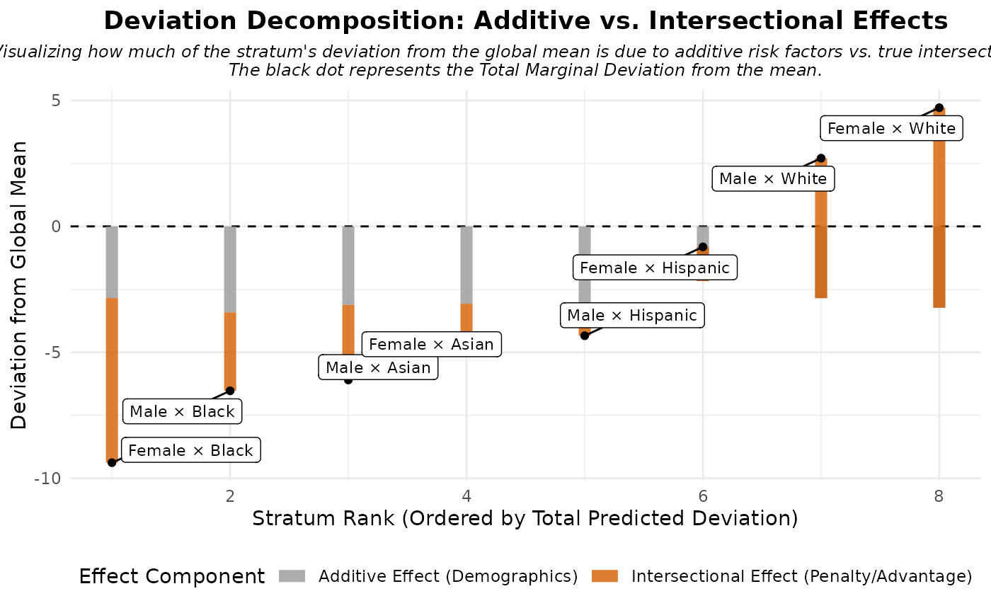
"predicted"– an intersection-size bar, a category matrix encoding each stratum's level on every dimension, and the predicted-value panel, all sharing one column order. Replaces the long intersectional axis labels with the matrix. Binary 0/1 dimensions show as a single present/absent row; multi-level factors get one row per level. Columns are ordered by intersection size (largest first) by default;order_by = "predicted_desc"gives the ranked caterpillar of"predicted"with the matrix in place of the text labels"effect_decomp": Visualizes additive vs intersectional deviation from global mean. Only the stratum random effect and, for a crossed-dimensions fit, the dimension random effects enter; a contextual random effect, or any other grouping, belongs to neither component and is left out of the deviations and the global mean, as it is from the
"predicted"values"prediction_deviation": Detailed deviation panels for individuals or strata
"context_vpc": Stratum vs. context variance bars for a contextual cross-classified fit (
fit_maihda(context = )); errors otherwise. For a crossed-dimensions fit with a context the between-stratum variance is drawn as its additive dimension and interaction bars"vpc_trajectory": Time-varying VPC/ICC curve for a longitudinal fit (
fit_maihda(id =, time =)); errors otherwise. For a longitudinal model"vpc"and"all"also route here"trajectories": Predicted per-stratum mean trajectories over time (longitudinal fits only)
"all": Generate all available plots (default if not specified)
- summary_obj
Optional maihda_summary object from
summary(). If NULL, will be computed.- n_strata
Maximum number of strata to display in the predicted plot. When there are more strata than this, the first
n_strata(in stratum order) are shown and the plot caption notes how many were omitted. Default is 50. Use NULL for all strata.- highlight_interactions
Highlight the strata that carry a credibly non-zero intersectional interaction (from
maihda_interactions) on the BLUP-based views ("effect_decomp","predicted","obs_vs_shrunken"); other views ignore it.FALSE(default) off;TRUEcomputes the flags withmaihda_interactions()defaults; or pass a multiple-testing method such as"BH"or amaihda_interactionsobject to reuse a specificconf_level/adjust. For the pure-interaction reading the model should be the adjusted (or crossed-dimensions) model – e.g. viaplot()on amaihdaanalysis, which routes these views to the adjusted model automatically. Which column of the screen drives the highlight set is governed byhighlight_by.- only_flagged
Show only the flagged strata rather than dimming the rest.
FALSE(default) keeps every stratum (flagged ones highlighted);TRUErestricts the"predicted"and"obs_vs_shrunken"views to the highlighted strata (those carrying a credibly non-zero interaction, or – underhighlight_by = "rope"– those classified ROPE-"relevant"), so a highlighted stratum is never hidden by then_stratacap. WhenTRUEandhighlight_interactionsis leftFALSE, the flags are computed withmaihda_interactionsdefaults; passhighlight_interactionsto choose theconf_level/adjust. A captioned empty panel is returned when no stratum is flagged. It does not apply to"effect_decomp"(whose waterfall exists to show each flagged stratum's place in the full distribution); that view stays highlighted. Independently of this argument, whenever interactions are highlighted then_stratacap on"predicted"becomes flag-aware: every flagged stratum is kept and the remaining slots are filled according toselect.- highlight_by
Which interaction-screen column defines the highlighted strata:
"flag"(default) uses the zero-centredflaggedcolumn (credibly non-zero interaction), preserving the historical behaviour;"rope"uses the equivalencedecisioncolumn, highlighting the strata classified"relevant"(interaction interval entirely outside the region of practical equivalence)."rope"requires a screen carrying adecisioncolumn: either passrope, or supply amaihda_interactionsobject built withrope; otherwise it errors.- rope
Equivalence region (a "smallest interaction of interest") forwarded to
maihda_interactionswhen the screen is computed here (i.e. whenhighlight_interactionsisTRUEor ap.adjustmethod name).NULL(default) adds no equivalence classification; a single positivedmeans the symmetric regionc(-d, d)on the latent (link) scale, or supplyc(lower, upper). Needed forhighlight_by = "rope"unless the suppliedmaihda_interactionsobject already carries adecisioncolumn. Ignored when a precomputedmaihda_interactionsobject is passed (its ownropeis used).- select
When the
n_stratacap must drop strata, which to keep:"order"(default; the first n_strata in stratum order, the historical behaviour) or"deviation"(the n_strata furthest from the reference line – largest|predicted - reference|, so the most extreme strata in both directions). Applies to"predicted"and, for a longitudinal fit,"trajectories"(where it keeps the strata whose trajectories swing furthest from the population curve). Flagged strata are always kept; this governs the fill and the unflagged case.selectchanges which strata appear; their left-to-right display order is a separate choice governed byorder_by.- order_by
For
type = "predicted"andtype = "upset", how to order the strata that are displayed (display-only – it does not change which strata are shown, that isn_strata/select, nor the predicted values, intervals, reference line, or highlighted set):"predicted_desc"orders from the highest predicted value to the lowest,"stratum"keeps the native stratum order,"predicted_asc"orders from lowest to highest,"deviation"orders by largest absolute deviation from the reference line (|predicted - reference|), and"size"orders by intersection (stratum) size, largest first. The default is per view:"predicted_desc"for"predicted"(labels run from the highest predicted value down) and"size"for"upset"(the UpSet convention, which also makes its intersection-size bar monotone). On the"upset"view the three value-based orders sort on the quantity the bottom panel actually shows, so they followquantity– withquantity = "interaction"they order by the stratum random effect and"deviation"measures the distance from zero. Combiningorder_by = "predicted_desc"withtype = "upset"gives the ranked caterpillar of the"predicted"view drawn against the UpSet category matrix instead of long text labels. Ignored by the other plot types.- quantity
For
type = "upset", which quantity the bottom panel shows:"predicted"(default) the stratum's predicted value (fixed + random effect) against the across-strata reference line, or"interaction"the stratum random effect (the BLUP) against zero – the deviation from the model's fixed prediction, which is the pure intersectional interaction when the dimension main effects are in the model (the adjusted model). Ignored by the other plot types.- ...
Additional arguments (not currently used).
Value
For a single type, a ggplot2 object that you can extend
with the usual + grammar (themes, labs(),
added layers, or a replacement fill/colour scale). Some types return a
richer object: "prediction_deviation" returns a patchwork of
two panels and "upset" a patchwork of three panels (theme
every panel at once with & theme_*()).
type = "all" returns a named list of ggplot2 objects.
Examples
# \donttest{
strata_result <- make_strata(maihda_sim_data, vars = c("gender", "race"))
model <- fit_maihda(health_outcome ~ age + (1 | stratum), data = strata_result$data)
# VPC plot
plot(model, type = "vpc")
 # Single-type plots are ggplot objects -- restyle them with ggplot2:
plot(model, type = "vpc") +
ggplot2::theme_classic() +
ggplot2::labs(title = "Variance partition, restyled")
# Single-type plots are ggplot objects -- restyle them with ggplot2:
plot(model, type = "vpc") +
ggplot2::theme_classic() +
ggplot2::labs(title = "Variance partition, restyled")
 # Generate all plots (a named list); pick one out to restyle it:
plots <- plot(model)
# Generate all plots (a named list); pick one out to restyle it:
plots <- plot(model)
 plots$predicted + ggplot2::theme_bw()
 # }
# }